R: Analysis of weather events impact on population health and economy.

Synopsis¶

This analysis involves exploring the U.S. National Oceanic and Atmospheric Administration's (NOAA) storm database.

This database tracks characteristics of major storms and weather events in the United States, including when and where they occur, as well as estimates of any fatalities, injuries, and property damage.

This analysis focuses on fatalities, injuries, property and crop damages to answer to the 2 following questions : Across the United States, which types of events (as indicated in the EVTYPE variable) are most harmful with respect to population health? Across the United States, which types of events have the greatest economic consequences?

Data Processing¶

The data comes in the form of a comma-separated-value file compressed via the bzip2.

We download it and unzip it in a ProjectData directory:

download.file("https://d396qusza40orc.cloudfront.net/repdata%2Fdata%2FStormData.csv.bz2", "FStormData.csv.bz2", 
    method = "curl", quiet = TRUE)

raw <- read.csv(bzfile("FStormData.csv.bz2"), sep = ",", quote = "\"", header = TRUE, stringsAsFactors = FALSE)
raw$BGN_DATE <- as.Date(raw$BGN_DATE, format = "%m/%d/%Y %H:%M:%S")
raw$END_DATE <- as.Date(raw$END_DATE, format = "%m/%d/%Y %H:%M:%S")

The Storm Events Database reports that all weather events are only recorded since 1996 (see http://www.ncdc.noaa.gov/stormevents/details.jsp).

    Event Types Available:
    Add more info about event types here. Link to collections page/tab when referencing data collection source.

    1. Tornado: From 1950 through 1954, only tornado events were recorded.

    2. Tornado, Thunderstorm Wind and Hail: From 1955 through 1992, only tornado, thunderstorm wind and hail events were keyed from the paper publications into digital data. From 1993 to 1995, only tornado, thunderstorm wind and hail events have been extracted from the Unformatted Text Files.

    3. All Event Types (48 from Directive 10-1605): From 1996 to present, 48 event types are recorded as defined in NWS Directive 10-1605.

Since we're reporting impacts from various weather events, we'll focus our study on data since 1996.

data <- raw[raw$BGN_DATE > "1996-01-01", ]
rm(raw)

Results¶

Weather events impact on population health across the United States since 1996

To study the weather events impact on poulation health, we examine the INJURIES AND FATALITIES columns of the dataset.

We compute the sum of total of injuries/fatalities by weather event type an store the values in a new dataset:

fat_by_ev <- aggregate(FATALITIES ~ EVTYPE, data = data, sum, na.rm = TRUE)
inj_by_ev <- aggregate(INJURIES ~ EVTYPE, data = data, sum, na.rm = TRUE)

For fatalities, the quantile function shows that only 1% of the values of the total of injuries/fatalities by event type are significant (> 326 fatalities, > 1635 injuries).

quantile(fat_by_ev$FATALITIES, probs = seq(0.9, 1, 0.01))

##     90%     91%     92%     93%     94%     95%     96%     97%     98%     99%    100% 
##    4.00    5.74    9.88   14.02   28.80   57.90   78.08  105.32  198.92  326.14 1797.00

quantile(inj_by_ev$INJURIES, probs = seq(0.9, 1, 0.01))

##      90%      91%      92%      93%      94%      95%      96%      97%      98%      99%     100% 
##    21.60    25.74    39.76    70.04    85.76   171.90   304.56   477.80  1034.84  1635.64 20667.00

We order the new datas by fatalities/injuries (decreasing order) and display the 10th first rows:

fat_temp <- fat_by_ev[order(fat_by_ev$FATALITIES, decreasing = TRUE), ][1:10, ]
colnames(fat_temp) <- c("event.type", "fatalities")
inj_temp <- inj_by_ev[order(inj_by_ev$INJURIES, decreasing = TRUE), ][1:10, ]
colnames(inj_temp) <- c("event.type", "injuries")
library(knitr)
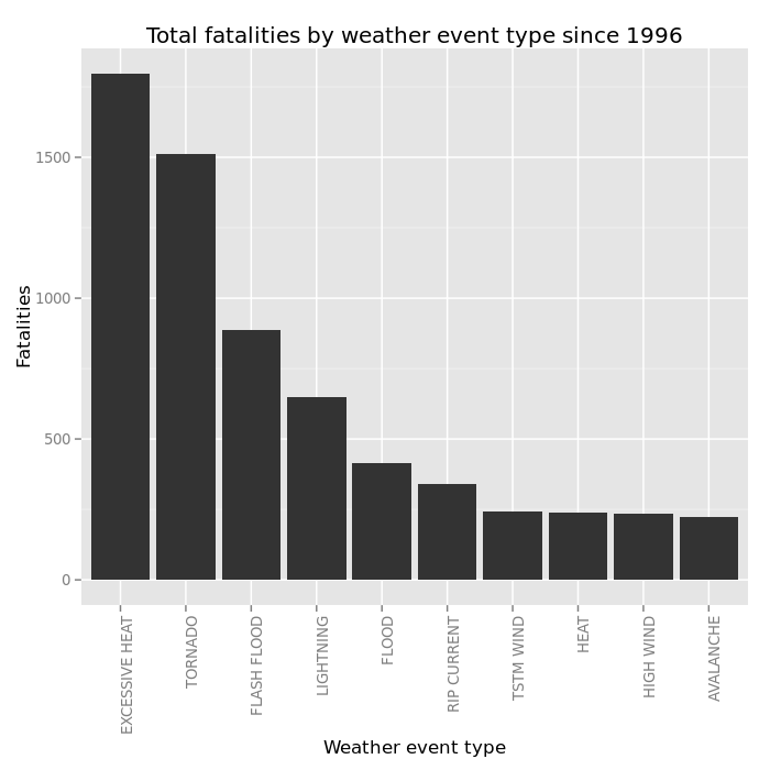
kable(fat_temp, caption = "Total fatalities by weather event type since 1996")

	event.type	fatalities
75	EXCESSIVE HEAT	1797
417	TORNADO	1511
96	FLASH FLOOD	887
213	LIGHTNING	650
99	FLOOD	414
286	RIP CURRENT	340
423	TSTM WIND	241
143	HEAT	237
161	HIGH WIND	235
16	AVALANCHE	223

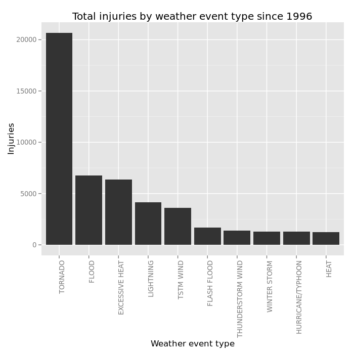
kable(inj_temp, caption = "Total injuries by weather event type since 1996")

	event.type	injuries
417	TORNADO	20667
99	FLOOD	6758
75	EXCESSIVE HEAT	6391
213	LIGHTNING	4140
423	TSTM WIND	3629
96	FLASH FLOOD	1674
413	THUNDERSTORM WIND	1400
496	WINTER STORM	1292
167	HURRICANE/TYPHOON	1275
143	HEAT	1222

Then plot the datas:

library(ggplot2)
ggplot(fat_temp, aes(reorder(factor(event.type), -fatalities), fatalities)) + geom_bar(stat = "identity") + 
    labs(x = "Weather event type", y = "Fatalities", title = "Total fatalities by weather event type since 1996") + 
    theme(axis.text.x = element_text(angle = 90, hjust = 1))

plot of chunk weather_events_impact_fatalities

ggplot(inj_temp, aes(reorder(factor(event.type), -injuries), injuries)) + geom_bar(stat = "identity") + 
    labs(x = "Weather event type", y = "Injuries", title = "Total injuries by weather event type since 1996") + 
    theme(axis.text.x = element_text(angle = 90, hjust = 1))

plot of chunk weather_events_impact_injuries

To go deeper, we can examine single weather types by having a closer look on their frequency/injuries and fatalities ratio :

library(plyr)
fat_ev_count <- count(data[data$FATALITIES > 0, ], vars = "EVTYPE")

temp <- merge(fat_ev_count, fat_by_ev, by = "EVTYPE")
temp$ratio <- temp$FATALITIES/temp$freq
colnames(temp) <- c("event.type", "event.frequency", "event.fatalities", "event.fatalities.ratio")
kable(temp[order(temp$event.frequency, decreasing = TRUE), ][1:30, ], caption = "Total fatalities by weather event type (ordered by frequency desc) since 1996")

	event.type	event.frequency	event.fatalities	event.fatalities.ratio
63	LIGHTNING	608	650	1.069079
27	FLASH FLOOD	584	887	1.518836
20	EXCESSIVE HEAT	564	1797	3.186170
92	TORNADO	459	1511	3.291939
74	RIP CURRENT	301	340	1.129568
28	FLOOD	270	414	1.533333
94	TSTM WIND	212	241	1.136793
75	RIP CURRENTS	179	202	1.128492
48	HIGH WIND	176	235	1.335227
1	AVALANCHE	173	223	1.289017
38	HEAT	133	237	1.781955
104	WINTER STORM	118	191	1.618644
90	THUNDERSTORM WIND	107	130	1.214953
85	STRONG WIND	90	103	1.144444
22	EXTREME COLD/WIND CHILL	87	125	1.436782
21	EXTREME COLD	86	113	1.313953
41	HEAVY SNOW	75	107	1.426667
11	COLD/WIND CHILL	74	95	1.283784
45	HIGH SURF	63	87	1.380952
39	HEAVY RAIN	59	94	1.593220
58	ICE STORM	51	82	1.607843
3	BLIZZARD	46	70	1.521739
29	FOG	35	60	1.714286
105	WINTER WEATHER	29	33	1.137931
101	WILDFIRE	28	75	2.678571
43	HEAVY SURF/HIGH SURF	27	42	1.555556
93	TROPICAL STORM	24	57	2.375000
49	HURRICANE	23	61	2.652174
98	URBAN/SML STREAM FLD	22	28	1.272727
50	HURRICANE/TYPHOON	19	64	3.368421

inj_ev_count <- count(data[data$INJURIES > 0, ], vars = "EVTYPE")
temp <- merge(inj_ev_count, inj_by_ev, by = "EVTYPE")
temp$ratio <- temp$INJURIES/temp$freq
colnames(temp) <- c("event.type", "event.frequency", "event.injuries", "event.injuries.ratio")
kable(temp[order(temp$event.frequency, decreasing = TRUE), ][1:30, ], caption = "Total Injuries by weather event type (ordered by frequency desc) since 1996")

	event.type	event.frequency	event.injuries	event.injuries.ratio
56	LIGHTNING	2250	4140	1.840000
85	TORNADO	1877	20667	11.010655
87	TSTM WIND	1492	3629	2.432306
83	THUNDERSTORM WIND	587	1400	2.385009
43	HIGH WIND	403	1083	2.687345
23	FLASH FLOOD	335	1674	4.997015
99	WILDFIRE	184	911	4.951087
34	HAIL	165	713	4.321212
17	EXCESSIVE HEAT	162	6391	39.450617
79	STRONG WIND	147	278	1.891156
101	WINTER STORM	144	1292	8.972222
24	FLOOD	142	6758	47.591549
98	WILD/FOREST FIRE	130	545	4.192308
68	RIP CURRENT	107	209	1.953271
1	AVALANCHE	105	156	1.485714
38	HEAVY SNOW	102	698	6.843137
69	RIP CURRENTS	84	294	3.500000
25	FOG	73	712	9.753425
37	HEAVY RAIN	73	230	3.150685
51	ICE STORM	53	318	6.000000
3	BLIZZARD	41	385	9.390244
15	DUST STORM	38	376	9.894737
36	HEAT	36	1222	33.944444
42	HIGH SURF	33	146	4.424242
102	WINTER WEATHER	30	343	11.433333
90	TSTM WIND/HAIL	26	95	3.653846
95	URBAN/SML STREAM FLD	26	79	3.038461
100	WIND	26	84	3.230769
86	TROPICAL STORM	23	338	14.695652
11	DENSE FOG	20	143	7.150000

Weather events economic impact across Unites States

We'll examine the property and crop damages columns (PROPDMG * 10^PROPDMGEXP and CROPDMG * 10^CROPDMGEXP, respectively) from the dataset.

We need to preprocess the data to convert PROPDMG and PROPDMGEXP into numbers, idem for CROPDMG and CROPDMGEXP.

Values for the CROPDMGEXP and PROPDMEXP are:

0 or blank
H for Hundred
K for Thousand
M for Million
B for Billion

Note: Except for these exponential values (H,K,M,B), there is some inexpected values : ? + - and numbers in the initial dataset. This values doesn't appear in the dataset filtered by BGN_DATE > 1996-01-01.

Let's check the repartition of the exponential categories:

table(data$CROPDMGEXP)

## 
##             B      K      M 
## 373047      4 278685   1771

table(data$PROPDMGEXP)

## 
##             0      B      K      M 
## 276166      1     32 369934   7374

We convert PROPDMG/PROPDMGEXP and CROPDMG/CROPDMGEXP pairs into numbers:

data$cropdmg.exp <- 1
data[data$CROPDMGEXP == "H", "cropdmg.exp"] <- 100
data[data$CROPDMGEXP == "K", "cropdmg.exp"] <- 1000
data[data$CROPDMGEXP == "M", "cropdmg.exp"] <- 10^6
data[data$CROPDMGEXP == "B", "cropdmg.exp"] <- 10^9
data$cropdmg.val <- data$CROPDMG * data$cropdmg.exp

data$propdmg.exp <- 1
data[data$PROPDMGEXP == "H", "propdmg.exp"] <- 100
data[data$PROPDMGEXP == "K", "propdmg.exp"] <- 1000
data[data$PROPDMGEXP == "M", "propdmg.exp"] <- 1e+06
data[data$PROPDMGEXP == "B", "propdmg.exp"] <- 1e+09
data$propdmg.val <- data$PROPDMG * data$propdmg.exp

We perform the same analysis as for weather type impact on population health:

crop_by_ev <- aggregate(cropdmg.val ~ EVTYPE, data = data, sum, na.rm = TRUE)
quantile(crop_by_ev$cropdmg.val, probs = seq(0.9, 1, 0.01))

##         90%         91%         92%         93%         94%         95%         96%         97% 
##       80000      522000     1830000     8518338    15105600    22067850    51986350   225801006 
##         98%         99%        100% 
##   611260434  1328471682 13367566000

prop_by_ev <- aggregate(propdmg.val ~ EVTYPE, data = data, sum, na.rm = TRUE)
quantile(prop_by_ev$propdmg.val, probs = seq(0.9, 1, 0.01))

##          90%          91%          92%          93%          94%          95%          96% 
##      6087080      7928162      9823200     19765792     40787880    117527100    551709366 
##          97%          98%          99%         100% 
##   1328347705   4595502763  14205618003 143944833550

crop_temp <- crop_by_ev[order(crop_by_ev$cropdmg.val, decreasing = TRUE), ][1:20, ]
colnames(crop_temp) <- c("event.type", "cropdmg.val")
prop_temp <- prop_by_ev[order(prop_by_ev$propdmg.val, decreasing = TRUE), ][1:20, ]
colnames(prop_temp) <- c("event.type", "propdmg.val")
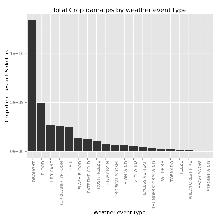
kable(crop_temp, caption = "Total crop damages in (US dollars) by weather event type")

	event.type	cropdmg.val
59	DROUGHT	13367566000
99	FLOOD	4974778400
166	HURRICANE	2741410000
167	HURRICANE/TYPHOON	2607872800
139	HAIL	2476029450
96	FLASH FLOOD	1334901700
81	EXTREME COLD	1288973000
108	FROST/FREEZE	1094086000
145	HEAVY RAIN	728169800
420	TROPICAL STORM	677711000
161	HIGH WIND	633561300
423	TSTM WIND	553915350
75	EXCESSIVE HEAT	492402000
413	THUNDERSTORM WIND	398331000
487	WILDFIRE	295472800
417	TORNADO	283425010
102	FREEZE	146225000
486	WILD/FOREST FIRE	106782330
150	HEAVY SNOW	71122100
330	STRONG WIND	64953500

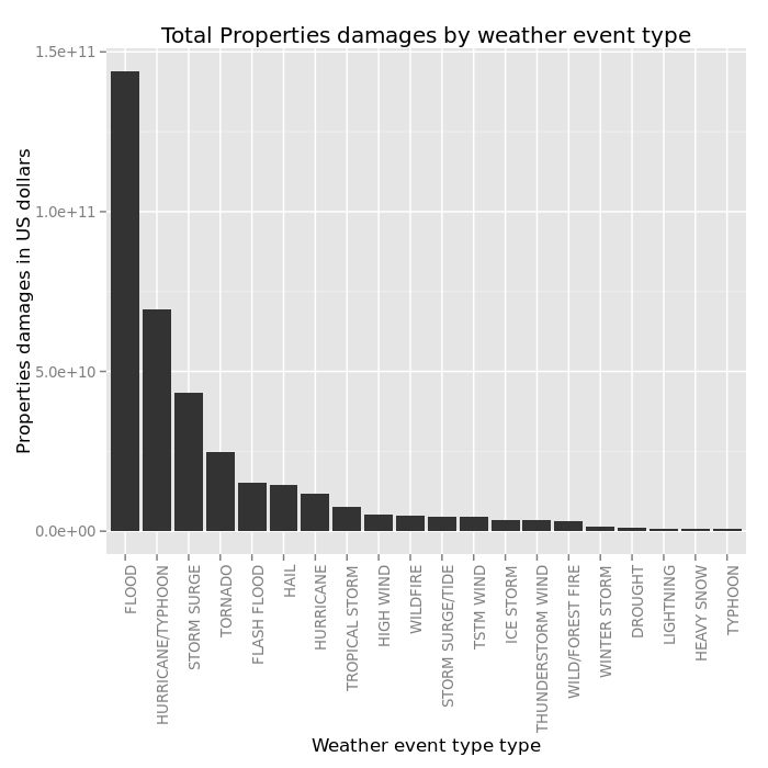
kable(prop_temp, caption = "Total property damages (in US dollars) by weather event type")

	event.type	propdmg.val
99	FLOOD	143944833550
167	HURRICANE/TYPHOON	69305840000
327	STORM SURGE	43193536000
417	TORNADO	24616905710
96	FLASH FLOOD	15222203910
139	HAIL	14595143420
166	HURRICANE	11812819010
420	TROPICAL STORM	7642475550
161	HIGH WIND	5247860360
487	WILDFIRE	4758667000
328	STORM SURGE/TIDE	4641188000
423	TSTM WIND	4478026440
191	ICE STORM	3642248810
413	THUNDERSTORM WIND	3382654440
486	WILD/FOREST FIRE	3001782500
496	WINTER STORM	1532733250
59	DROUGHT	1046101000
213	LIGHTNING	743077080
150	HEAVY SNOW	634417540
437	TYPHOON	600230000

ggplot(crop_temp, aes(reorder(factor(event.type), -cropdmg.val), cropdmg.val)) + geom_bar(stat = "identity") + 
    labs(x = "Weather event type", y = "Crop damages in US dollars", title = "Total Crop damages by weather event type") + 
    theme(axis.text.x = element_text(angle = 90, hjust = 1))

plot of chunk weather_events_impact_crop_damages

ggplot(prop_temp, aes(reorder(factor(event.type), -propdmg.val), propdmg.val)) + geom_bar(stat = "identity") + 
    labs(x = "Weather event type type", y = "Properties damages in US dollars", title = "Total Properties damages by weather event type") + 
    theme(axis.text.x = element_text(angle = 90, hjust = 1))

plot of chunk weather_events_impact_properties_damages

and we check damages ratio by event type:

crop_ev_count <- count(data[data$cropdmg.val > 0, ], vars = "EVTYPE")
temp <- merge(crop_ev_count, crop_by_ev, by = "EVTYPE")
temp$ratio <- temp$cropdmg.val/temp$freq
colnames(temp) <- c("event.type", "event.frequency", "event.cropdamages", "event.cropdamages.ratio")
kable(temp[order(temp$event.frequency, decreasing = TRUE), ][1:20, ], caption = "Total crop domages (in US dollars) by weather event type (ordered by frequency desc) since 1996")

	event.type	event.frequency	event.cropdamages	event.cropdamages.ratio
22	HAIL	8100	2476029450	305682.65
46	TSTM WIND	3440	553915350	161021.90
14	FLASH FLOOD	1845	1334901700	723523.96
15	FLOOD	1599	4974778400	3111180.99
44	TORNADO	1254	283425010	226016.75
43	THUNDERSTORM WIND	924	398331000	431094.16
4	DROUGHT	243	13367566000	55010559.67
27	HIGH WIND	200	633561300	3167806.50
25	HEAVY RAIN	123	728169800	5920079.67
53	URBAN/SML STREAM FLD	112	8488100	75786.61
17	FROST/FREEZE	102	1094086000	10726333.33
42	STRONG WIND	94	64953500	690994.68
47	TSTM WIND/HAIL	89	64696250	726924.16
56	WILDFIRE	89	295472800	3319919.10
33	LIGHTNING	74	6898440	93222.16
45	TROPICAL STORM	59	677711000	11486627.12
28	HURRICANE	47	2741410000	58327872.34
9	EXTREME COLD	46	1288973000	28021152.17
55	WILD/FOREST FIRE	35	106782330	3050923.71
29	HURRICANE/TYPHOON	33	2607872800	79026448.48

prop_ev_count <- count(data[data$propdmg.val > 0, ], vars = "EVTYPE")
temp <- merge(prop_ev_count, prop_by_ev, by = "EVTYPE")
temp$ratio <- temp$propdmg.val/temp$freq
colnames(temp) <- c("event.type", "event.frequency", "event.propdamages", "event.propdamages.ratio")
kable(temp[order(temp$event.frequency, decreasing = TRUE), ][1:20, ], caption = "Total property damages (in US dollars) by weather event type (ordered by frequency desc) since 1996")

	event.type	event.frequency	event.propdamages	event.propdamages.ratio
142	TSTM WIND	60331	4478026440	74224.30
137	THUNDERSTORM WIND	42726	3382654440	79170.87
65	HAIL	20002	14595143420	729684.20
39	FLASH FLOOD	18647	15222203910	816335.28
139	TORNADO	11847	24616905710	2077902.06
41	FLOOD	9086	143944833550	15842486.63
96	LIGHTNING	8744	743077080	84981.37
74	HIGH WIND	5217	5247860360	1005915.35
131	STRONG WIND	3206	174741450	54504.51
166	WINTER STORM	1344	1532733250	1140426.53
68	HEAVY SNOW	943	634417540	672765.15
67	HEAVY RAIN	906	584864440	645545.74
163	WILDFIRE	723	4758667000	6581835.41
157	URBAN/SML STREAM FLD	670	58309650	87029.33
84	ICE STORM	594	3642248810	6131732.00
141	TROPICAL STORM	390	7642475550	19596091.15
152	TSTM WIND/HAIL	380	44320500	116632.89
167	WINTER WEATHER	373	20866000	55941.02
162	WILD/FOREST FIRE	303	3001782500	9906872.94
88	LAKE-EFFECT SNOW	194	40115000	206778.35

Conclusions¶

Wheater events impact on population health Our analysys shows that since 1996:

The "Tornado" event caused the most injuries
Both the "Tornado" and "Excessive heat" events caused the most fatalities

From the frequency/ratio table, we can notice that:

The "Lightning", "Flash Flood" and "Excessive Heat" are the most frequent events regarding events causing fatalities
The "Lightning", "Tornado" and "TSM Wind" are the most frequent events regarding events causing injuries
The "Excessive heat", "Flood" and "Heat", have a very high ratio regarding injuries

Wheater events impact on economy Our analysys shows that since 1996:

The "Drought" event caused the most crop damages
The "Flood" events caused the most property damages

From the frequency/ratio table, we can notice that:

The "Hail" event is the most frequent event regarding events causing crop damages
The "TSTM Wind" event is the most frequent event regarding events causing property damages
The "Drought" and "Hurricane" events have a very high crop damages ratio
The "Flood" and "Tropical storm" events have a very high property damages ratio

Synopsis¶

Data Processing¶

Results¶

Conclusions¶

Related Posts: