This is my note on swirl course Regression Model : Multivariable Examples 3.
We'll use the hunger dataset from the course:
download.file("https://raw.githubusercontent.com/swirldev/swirl_courses/master/Regression_Models/MultiVar_Examples3/hunger.csv",
    "hunger.csv", method = "curl", quiet = T)
hunger <- read.csv("hunger.csv")
head(hunger)
##    X                              Indicator Data.Source PUBLISH.STATES Year WHO.region  Country
## 1  8 Children aged <5 years underweight (%) NLIS_310044      Published 1986     Africa  Senegal
## 2 11 Children aged <5 years underweight (%) NLIS_310095      Published 1989     Africa   Uganda
## 3 13 Children aged <5 years underweight (%) NLIS_310138      Published 1988     Africa Zimbabwe
## 4 16 Children aged <5 years underweight (%) NLIS_310044      Published 1986     Africa  Senegal
## 5 18 Children aged <5 years underweight (%) NLIS_310095      Published 1989     Africa   Uganda
## 6 21 Children aged <5 years underweight (%) NLIS_310138      Published 1988     Africa Zimbabwe
##      Sex Display.Value Numeric Low High Comments
## 1   Male          19.3    19.3  NA   NA       NA
## 2 Female          19.1    19.1  NA   NA       NA
## 3 Female           7.2     7.2  NA   NA       NA
## 4 Female          15.3    15.3  NA   NA       NA
## 5   Male          20.4    20.4  NA   NA       NA
## 6   Male           8.7     8.7  NA   NA       NA
The Numeric column gives the percentage of children under age 5 who were underweight when that sample was taken.
We fit a simple linear regression for Numeric (outcome) on Year:
fit <- lm(Numeric ~ Year, hunger)
summary(fit)
##
## Call:
## lm(formula = Numeric ~ Year, data = hunger)
##
## Residuals:
##     Min      1Q  Median      3Q     Max
## -24.621 -11.196  -1.994   7.085  45.039
##
## Coefficients:
##              Estimate Std. Error t value Pr(>|t|)
## (Intercept) 634.47966  121.14460   5.237 2.01e-07 ***
## Year         -0.30840    0.06053  -5.095 4.21e-07 ***
## ---
## Signif. codes:  0 '***' 0.001 '**' 0.01 '*' 0.05 '.' 0.1 ' ' 1
##
## Residual standard error: 13.23 on 946 degrees of freedom
## Multiple R-squared:  0.02671,    Adjusted R-squared:  0.02568
## F-statistic: 25.96 on 1 and 946 DF,  p-value: 4.209e-07
As time goes on, the rate of hunger decreases.
The intercept of the model represents the percentage of hungry children at year 0.
Let's look at the rates of hunger for the different genders to see how, or even if, they differ:
lmF <- lm(Numeric[hunger$Sex == "Female"] ~ Year[hunger$Sex == "Female"], data = hunger)
summary(lmF)
##
## Call:
## lm(formula = Numeric[hunger$Sex == "Female"] ~ Year[hunger$Sex ==
##     "Female"], data = hunger)
##
## Residuals:
##     Min      1Q  Median      3Q     Max
## -23.228 -10.638  -1.959   6.859  46.146
##
## Coefficients:
##                               Estimate Std. Error t value Pr(>|t|)
## (Intercept)                  603.50580  167.53201   3.602 0.000349 ***
## Year[hunger$Sex == "Female"]  -0.29340    0.08371  -3.505 0.000500 ***
## ---
## Signif. codes:  0 '***' 0.001 '**' 0.01 '*' 0.05 '.' 0.1 ' ' 1
##
## Residual standard error: 12.94 on 472 degrees of freedom
## Multiple R-squared:  0.02537,    Adjusted R-squared:  0.0233
## F-statistic: 12.29 on 1 and 472 DF,  p-value: 5e-04
lmM <- lm(Numeric[hunger$Sex == "Male"] ~ Year[hunger$Sex == "Male"], data = hunger)
summary(lmM)
##
## Call:
## lm(formula = Numeric[hunger$Sex == "Male"] ~ Year[hunger$Sex ==
##     "Male"], data = hunger)
##
## Residuals:
##     Min      1Q  Median      3Q     Max
## -25.913 -11.741  -1.832   7.399  42.255
##
## Coefficients:
##                             Estimate Std. Error t value Pr(>|t|)
## (Intercept)                665.45352  174.50726   3.813 0.000155 ***
## Year[hunger$Sex == "Male"]  -0.32340    0.08719  -3.709 0.000233 ***
## ---
## Signif. codes:  0 '***' 0.001 '**' 0.01 '*' 0.05 '.' 0.1 ' ' 1
##
## Residual standard error: 13.48 on 472 degrees of freedom
## Multiple R-squared:  0.02832,    Adjusted R-squared:  0.02626
## F-statistic: 13.76 on 1 and 472 DF,  p-value: 0.0002328
We plot the data points and fitted lines using different colors to distinguish between males (blue) and females (pink).
plot(hunger$Year, hunger$Numeric, type = "n")
points(hunger$Year, hunger$Numeric, pch = 19, col = ((hunger$Sex == "Female") * 1 + 125))
lines(hunger$Year[hunger$Sex == "Male"], lmM$fitted, col = "blue", lwd = 3)
lines(hunger$Year[hunger$Sex == "Female"], lmF$fitted, col = "red", lwd = 3)
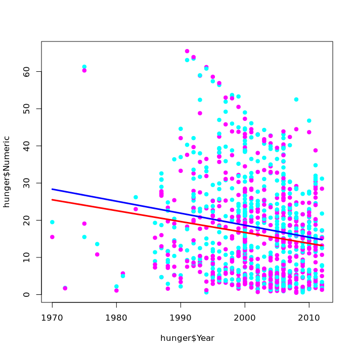
We can see from the plot that the lines are not exactly parallel. On the right side of the graph (around the year 2010) they are closer together than on the left side (around 1970). Slopes are -0.29340 for femals, -0.32340 for males.
Now instead of separating the data by subsetting the samples by gender, we'll use gender as another predictor to create the linear model:
lmBoth <- lm(Numeric ~ Year + Sex, data = hunger)
summary(lmBoth)
##
## Call:
## lm(formula = Numeric ~ Year + Sex, data = hunger)
##
## Residuals:
##     Min      1Q  Median      3Q     Max
## -25.472 -11.297  -1.848   7.058  45.990
##
## Coefficients:
##             Estimate Std. Error t value Pr(>|t|)
## (Intercept) 633.5283   120.8950   5.240 1.98e-07 ***
## Year         -0.3084     0.0604  -5.106 3.99e-07 ***
## SexMale       1.9027     0.8576   2.219   0.0267 *
## ---
## Signif. codes:  0 '***' 0.001 '**' 0.01 '*' 0.05 '.' 0.1 ' ' 1
##
## Residual standard error: 13.2 on 945 degrees of freedom
## Multiple R-squared:  0.03175,    Adjusted R-squared:  0.0297
## F-statistic: 15.49 on 2 and 945 DF,  p-value: 2.392e-07
Notice that Male and Female are factors (factors are treated in alphabetic order, so reference, here, is the Female group).
The intercept represents the percentage of hungry females at year 0.
The estimate for the factor Male 1.9027 is a distance from the intercept (the estimate of the reference group Female). So the percentage of hungry males at year 0 is the sum of the intercept and the male estimate, ie. 633.5283 + 1.9027 = 635.431
The estimate for hunger$Year represents the annual decrease in percentage of both gender.
In the plot, the red line will have the female intercept and the blue line will have the male intercept:
plot(hunger$Year, hunger$Numeric, pch = 19)
points(hunger$Year, hunger$Numeric, pch = 19, col = ((hunger$Sex == "Female") * 1 + 125))
abline(c(lmBoth$coeff[1], lmBoth$coeff[2]), col = "red", lwd = 3)
abline(c(lmBoth$coeff[1] + lmBoth$coeff[3], lmBoth$coeff[2]), col = "blue", lwd = 3)
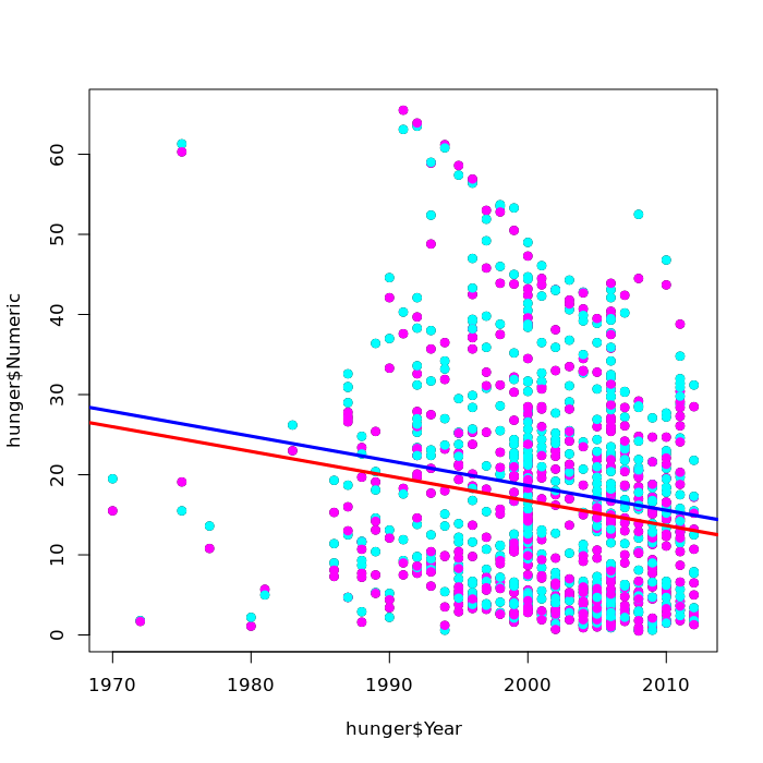
The lines are parallels (since, they have the same slope lmBoth$coeff[2]).
Now we'll consider the interaction between year and gender to see how that affects changes in rates of hunger:
lmInter <- lm(Numeric ~ Year + Sex + Sex * Year, data = hunger)
summary(lmInter)
##
## Call:
## lm(formula = Numeric ~ Year + Sex + Sex * Year, data = hunger)
##
## Residuals:
##     Min      1Q  Median      3Q     Max
## -25.913 -11.248  -1.853   7.087  46.146
##
## Coefficients:
##               Estimate Std. Error t value Pr(>|t|)
## (Intercept)  603.50580  171.05519   3.528 0.000439 ***
## Year          -0.29340    0.08547  -3.433 0.000623 ***
## SexMale       61.94772  241.90858   0.256 0.797946
## Year:SexMale  -0.03000    0.12087  -0.248 0.804022
## ---
## Signif. codes:  0 '***' 0.001 '**' 0.01 '*' 0.05 '.' 0.1 ' ' 1
##
## Residual standard error: 13.21 on 944 degrees of freedom
## Multiple R-squared:  0.03181,    Adjusted R-squared:  0.02874
## F-statistic: 10.34 on 3 and 944 DF,  p-value: 1.064e-06
The percentage of hungry females at year 0 is 603.5058.
The percentage of hungry males at year 0 is 665.4535 (603.50580 + 61.94772).
The annual change (decrease) in percentage of hungry females is 0.29340.
The estimate associated with Year:SexMale represents the distance of the annual change in percent of males from that of females.
The annual change in percentage of hungry males is -0.32340 (-0.29340 - 0.03000).
plot(hunger$Year, hunger$Numeric, pch = 19)
points(hunger$Year, hunger$Numeric, pch = 19, col = ((hunger$Sex == "Male") * 1 + 125))
abline(c(lmInter$coeff[1], lmInter$coeff[2]), col = "red", lwd = 3)
abline(c(lmInter$coeff[1] + lmInter$coeff[3], lmInter$coeff[2] + lmInter$coeff[4]), col = "blue", lwd = 3)
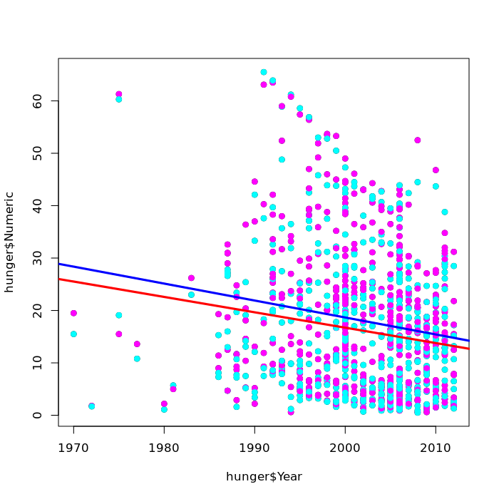
The lines are not parallel and will eventually intersect. The Male blue line indicates a faster rate of change.
Here we're dealing with an interaction between factors.
Suppose we have two interacting predictors and one of them is held constant.
The expected change in the outcome for a unit change in the other predictor is the coefficient of that changing predictor + the coefficient of the interaction * the value of the predictor held constant.
For example, let's the model be : \(H_i = b_0 + (b_1*I_i) + (b_2*Y_i)+ (b_3*I_i*Y_i)\) with H the outcomes, I's and Y's the predictors and b's the estimated coefficients of the predictors.
If I is fixed at a value, 5 and Y varies, \(b_2 + b3*5\) represents the change in H per unit change in Y given that I is fixed at 5.