The CLT Theorem:
The distribution of sample statistics (e.g. mean) is approximatively normal, regardless of the underlying distribution, with mean = \(\mu\) and variance = \(\sigma^2\)
To experiment this theory, we've built a matrix with 40 exponentials (we take lambda=0.2) x 1000 and compute the mean of each row, storing the result in a means vector:
set.seed(1234)
n <- 40
nosim <- 1000
lambda <- 0.2
means <- apply(matrix(rexp(nosim * n, lambda), nosim), 1, mean)
head(means)
## [1] 4.602510 6.017790 5.463686 4.176755 7.144672 4.427567
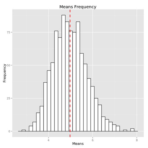
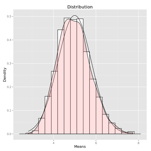
and plot an histogram of the means vector and the density distribution:
library(ggplot2)
dat <- data.frame(x = 1:nosim, y = means)

ggplot(dat, aes(x = y)) + geom_histogram(colour = "black", fill = "white") +
    geom_vline(aes(xintercept = mean(y)), color = "red", linetype = "dashed",
        size = 1) + labs(x = "Means", y = "Frequency", title = "Means Frequency")

ggplot(dat, aes(x = y)) + geom_histogram(binwidth = 0.3, colour = "black", fill = "white",
    aes(y = ..density..)) + stat_function(fun = dnorm, args = list(mean = 1/lambda,
    sd = 1/lambda/sqrt(n))) + labs(x = "Means", y = "Dendity", title = "Distribution") +
    geom_density(alpha = 0.2, fill = "#FF6666")

To confirm this distribution fits the normal distribution, we've draw the hump of the density of a random variable normally distributed with a mean \(1/\lambda\) and a standard deviation \(\frac{1/\lambda}{\sqrt{n}}\).