scikit-learn: Classification Algorithms on Iris Dataset

Source available on Nbviewer.

%matplotlib inline
import matplotlib.pyplot as plt
import numpy as np
from matplotlib.colors import ListedColormap

scikit-learn comes with a few standard datasets, for instance the iris and digits datasets for classification.
The iris dataset consists of measurements of three different species of irises.
scikit-learn embeds a copy of the iris CSV file along with a helper function to load it into numpy arrays.

from sklearn.datasets import load_iris
iris = load_iris()

iris.keys()

['target_names', 'data', 'target', 'DESCR', 'feature_names']

print iris.data.shape
print iris.target.shape

(150, 4)
(150,)

Exploring the dataset¶

The target classes to predict are iris classification:

setosa
versicolor
virginica

iris.target_names

array(['setosa', 'versicolor', 'virginica'], 
      dtype='|S10')

The features in the iris dataset are :

sepal length
sepal width
petal length
petal width

iris.feature_names

['sepal length (cm)',
 'sepal width (cm)',
 'petal length (cm)',
 'petal width (cm)']

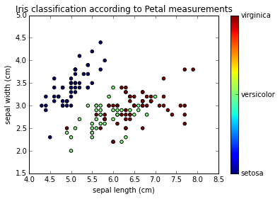
x_index = 2 #Petal Length
y_index = 3 #Petal Width
iris.data[:,x_index] # Petal Length values

array([ 1.4,  1.4,  1.3,  1.5,  1.4,  1.7,  1.4,  1.5,  1.4,  1.5,  1.5,
        1.6,  1.4,  1.1,  1.2,  1.5,  1.3,  1.4,  1.7,  1.5,  1.7,  1.5,
        1. ,  1.7,  1.9,  1.6,  1.6,  1.5,  1.4,  1.6,  1.6,  1.5,  1.5,
        1.4,  1.5,  1.2,  1.3,  1.5,  1.3,  1.5,  1.3,  1.3,  1.3,  1.6,
        1.9,  1.4,  1.6,  1.4,  1.5,  1.4,  4.7,  4.5,  4.9,  4. ,  4.6,
        4.5,  4.7,  3.3,  4.6,  3.9,  3.5,  4.2,  4. ,  4.7,  3.6,  4.4,
        4.5,  4.1,  4.5,  3.9,  4.8,  4. ,  4.9,  4.7,  4.3,  4.4,  4.8,
        5. ,  4.5,  3.5,  3.8,  3.7,  3.9,  5.1,  4.5,  4.5,  4.7,  4.4,
        4.1,  4. ,  4.4,  4.6,  4. ,  3.3,  4.2,  4.2,  4.2,  4.3,  3. ,
        4.1,  6. ,  5.1,  5.9,  5.6,  5.8,  6.6,  4.5,  6.3,  5.8,  6.1,
        5.1,  5.3,  5.5,  5. ,  5.1,  5.3,  5.5,  6.7,  6.9,  5. ,  5.7,
        4.9,  6.7,  4.9,  5.7,  6. ,  4.8,  4.9,  5.6,  5.8,  6.1,  6.4,
        5.6,  5.1,  5.6,  6.1,  5.6,  5.5,  4.8,  5.4,  5.6,  5.1,  5.1,
        5.9,  5.7,  5.2,  5. ,  5.2,  5.4,  5.1])

iris.target # Iris Classification values

array([0, 0, 0, 0, 0, 0, 0, 0, 0, 0, 0, 0, 0, 0, 0, 0, 0, 0, 0, 0, 0, 0, 0,
       0, 0, 0, 0, 0, 0, 0, 0, 0, 0, 0, 0, 0, 0, 0, 0, 0, 0, 0, 0, 0, 0, 0,
       0, 0, 0, 0, 1, 1, 1, 1, 1, 1, 1, 1, 1, 1, 1, 1, 1, 1, 1, 1, 1, 1, 1,
       1, 1, 1, 1, 1, 1, 1, 1, 1, 1, 1, 1, 1, 1, 1, 1, 1, 1, 1, 1, 1, 1, 1,
       1, 1, 1, 1, 1, 1, 1, 1, 2, 2, 2, 2, 2, 2, 2, 2, 2, 2, 2, 2, 2, 2, 2,
       2, 2, 2, 2, 2, 2, 2, 2, 2, 2, 2, 2, 2, 2, 2, 2, 2, 2, 2, 2, 2, 2, 2,
       2, 2, 2, 2, 2, 2, 2, 2, 2, 2, 2, 2])

formatter = plt.FuncFormatter(lambda i, *args: iris.target_names[int(i)])

plt.scatter(iris.data[:, x_index], iris.data[:, y_index],
            c=iris.target)
plt.colorbar(ticks=[0, 1, 2], format=formatter)
plt.xlabel(iris.feature_names[x_index])
plt.ylabel(iris.feature_names[y_index])
plt.title("Iris classification according to Petal measurements")

png

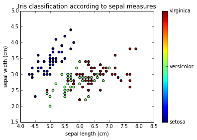
x_index = 0 # Sepal Lenght
y_index = 1 # Sepal Width
formatter = plt.FuncFormatter(lambda i, *args: iris.target_names[int(i)])

plt.scatter(iris.data[:, x_index], iris.data[:, y_index],
            c=iris.target)
plt.colorbar(ticks=[0, 1, 2], format=formatter)
plt.xlabel(iris.feature_names[x_index])
plt.ylabel(iris.feature_names[y_index])
plt.title("Iris classification according to sepal measurements")

png

Using classification algorithm¶

KNeighborsClassifier¶

The simplest possible classifier is the nearest neighbor.

Fitting the model¶

from sklearn import neighbors
knn = neighbors.KNeighborsClassifier(n_neighbors=1)
knn.fit(iris.data, iris.target)

KNeighborsClassifier(algorithm='auto', leaf_size=30, metric='minkowski',
           metric_params=None, n_neighbors=1, p=2, weights='uniform')

Doing a predicition¶

result = knn.predict([[3, 5, 4, 2],]) # What is the iris class for 3cm x 5cm sepal and 4cm x 2cm petal?
print iris.target_names[result]

['virginica']

Exploring the results¶

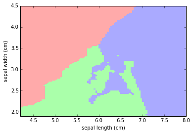
Let's draw the classification region according to sepal measurements.
First, let's fit the model using the two first features only:

X = iris.data[:, :2] #Working with the two first features : sepal length and sepal width
y = iris.target

knn = neighbors.KNeighborsClassifier(n_neighbors=3)
knn.fit(X, y)

KNeighborsClassifier(algorithm='auto', leaf_size=30, metric='minkowski',
           metric_params=None, n_neighbors=3, p=2, weights='uniform')

Then, let's build a input data matrix containing continuous values of sepal length and width (from min to max) and aply the predict function to it:

x_min, x_max = X[:, 0].min() - .1, X[:, 0].max() + .1 #min and max sepal length
y_min, y_max = X[:, 1].min() - .1, X[:, 1].max() + .1 #min and max sepal width
xx, yy = np.meshgrid(np.linspace(x_min, x_max, 100),
                     np.linspace(y_min, y_max, 100))
Z = knn.predict(np.c_[xx.ravel(), yy.ravel()])
Z = Z.reshape(xx.shape)

Let's put the result into a color plot:

plt.figure()

# Create color maps for 3-class classification problem
from matplotlib.colors import ListedColormap
cmap_light = ListedColormap(['#FFAAAA', '#AAFFAA', '#AAAAFF'])
cmap_bold = ListedColormap(['#FF0000', '#00FF00', '#0000FF'])

# Plot Classification Map
plt.pcolormesh(xx, yy, Z, cmap=cmap_light, )
plt.xlabel('sepal length (cm)')
plt.ylabel('sepal width (cm)')
plt.axis('tight')

(4.2000000000000002, 8.0, 1.8999999999999999, 4.5)

png

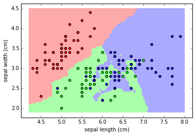
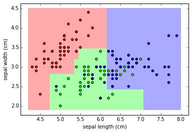
Let's add the actual values of iris sepal lenght/width vs classification to the color map:

plt.pcolormesh(xx, yy, Z, cmap=cmap_light)
# Add training points
plt.scatter(X[:, 0], X[:, 1], c=y, cmap=cmap_bold)
plt.xlabel('sepal length (cm)')
plt.ylabel('sepal width (cm)')
plt.axis('tight')

(4.0099999999999998, 8.1899999999999995, 1.77, 4.6299999999999999)

png

Support Vector Classifier (SVC)¶

from sklearn import svm

clf = svm.LinearSVC(loss = 'l2')

Fitting the model¶

clf.fit(iris.data, iris.target)

LinearSVC(C=1.0, class_weight=None, dual=True, fit_intercept=True,
     intercept_scaling=1, loss='l2', multi_class='ovr', penalty='l2',
     random_state=None, tol=0.0001, verbose=0)

Doing a predicition¶

result = clf.predict([[3, 5, 4, 2],])# What is the iris class for 3cm x 5cm sepal and 4cm x 2cm petal?
print iris.target_names[result]

['virginica']

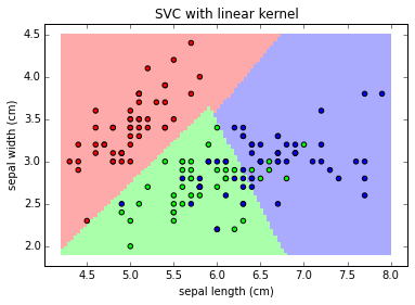
Exploring different classifiers (kernels)¶

X = iris.data[:, :2] #Working with the two first features : sepal length and sepal width
y = iris.target

def plot_class_map(clf, X, y, title="", **params):
    C = 1.0  # SVM regularization parameter

    clf.fit(X, y)
    x_min, x_max = X[:, 0].min() - .1, X[:, 0].max() + .1
    y_min, y_max = X[:, 1].min() - .1, X[:, 1].max() + .1
    xx, yy = np.meshgrid(np.linspace(x_min, x_max, 100),
                         np.linspace(y_min, y_max, 100))
    Z = clf.predict(np.c_[xx.ravel(), yy.ravel()])
    Z = Z.reshape(xx.shape)

    plt.figure()

    from matplotlib.colors import ListedColormap
    cmap_light = ListedColormap(['#FFAAAA', '#AAFFAA', '#AAAAFF'])
    cmap_bold = ListedColormap(['#FF0000', '#00FF00', '#0000FF'])
    plt.pcolormesh(xx, yy, Z, cmap=cmap_light)
    #Plot training points as well
    plt.scatter(X[:, 0], X[:, 1], c=y, cmap=cmap_bold)
    plt.xlabel('sepal length (cm)')
    plt.ylabel('sepal width (cm)')
    plt.axis('tight')
    plt.title(title)

# Linear
clf = svm.SVC(kernel='linear')
plot_class_map(clf, X, y, 'SVC with linear kernel')

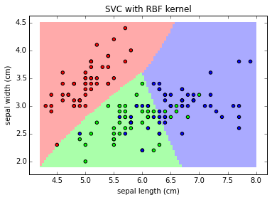
# RBF
clf = svm.SVC(kernel='rbf')
plot_class_map(clf, X, y, 'SVC with linear kernel')

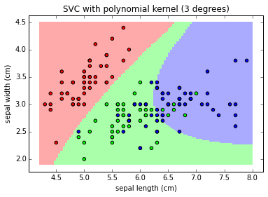
# RBF 
clf = svm.SVC(kernel='poly', degree=3)
plot_class_map(clf, X, y, 'SVC with polynomial kernel (3 degrees)')

png

Note:

The linear models LinearSVC() and SVC(kernel='linear') yield slightly different decision boundaries. This can be a consequence of the following differences:

LinearSVC minimizes the squared hinge loss while SVC minimizes the regular hinge loss.
LinearSVC uses the One-vs-All (also known as One-vs-Rest) multiclass reduction while SVC uses the One-vs-One multiclass reduction.

clf = svm.SVC(kernel="linear")
clf.fit(iris.data, iris.target)
result = clf.predict([[3, 5, 4, 2],])# What is the iris class for 3cm x 5cm sepal and 4cm x 2cm petal?
print iris.target_names[result]

['versicolor']

Random Forest¶

from sklearn.tree import DecisionTreeClassifier

clf = DecisionTreeClassifier()

Fitting the model¶

clf.fit(iris.data, iris.target)

DecisionTreeClassifier(compute_importances=None, criterion='gini',
            max_depth=None, max_features=None, max_leaf_nodes=None,
            min_density=None, min_samples_leaf=1, min_samples_split=2,
            random_state=None, splitter='best')

Doing a predicition¶

result = clf.predict([[3, 5, 4, 2],])# What is the iris class for 3cm x 5cm sepal and 4cm x 2cm petal?
print iris.target_names[result]

['versicolor']

Decision Trees and over-fitting¶

X = iris.data[:, :2] #Working with the two first features : sepal length and sepal width
y = iris.target
clf.fit(X,y)

plot_class_map(clf, X, y)

png

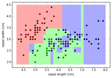
The issue with RF is it's tending to overfit the data.
hey are flexible enough that they can learn the structure of the noise in the data rather than the signal.

clf = DecisionTreeClassifier(max_depth=4)
clf.fit(X,y)
plot_class_map(clf, X, y)

png

The model obtained by limiting tree depth is a much better fit to the data.

Exploring the dataset¶

Using classification algorithm¶

KNeighborsClassifier¶

Fitting the model¶

Doing a predicition¶

Exploring the results¶

Support Vector Classifier (SVC)¶

Fitting the model¶

Doing a predicition¶

Exploring different classifiers (kernels)¶

Random Forest¶

Fitting the model¶

Doing a predicition¶

Decision Trees and over-fitting¶

Related Posts: